NFL Player Analysis
Which NFL players are poised to have breakout seasons next year? Which of last year's stars are going to regress? Do the league veterans have much more gas left in the tank?
Gridiron football fans ask themselves these questions at the outset of every NFL season. But questions like these are much more pressing if you have to manage a team in any capacity. Whether you're competing in a fantasy football league, assembling a competitive high school roster, recruiting for college athletics, or managing a professional club, accurately assessing player performance and potential is key to fielding the best possible team.
The Cogynt platform is ideally suited to solve this kind of problem. With its ability to accurately calculate risk and manage unknowns, Cogynt can help provide the clearest possible picture from the available data.
In this exercise, we use Cogynt to analyze quarterback (QB) statistics throughout a season to gauge their potential upside or downside if signed the following season. The model uses data scraped from Pro Football Reference for the 2019 NFL season.
For now, we only analyze QBs to keep the scope of the model manageable. We also use an older season for this exercise so that we can compare the model's findings to the way things really turned out in the 2020 season.
Requirements
This project assumes you have access to:
If you need access to Cogynt, please contact Cogility.
Building the Model
Let's look at how to build our proposed model in Cogynt.
Before you begin, be sure to:
- Create a new project in Cogynt Authoring.
- Gather all the data you need from Pro Football Reference.
- Upload your data to Cogynt as a CSV file.
Statistics to Evaluate
Now that Cogynt has data to work with, we need to tell it what separates the good QBs from the bad. This means we have to build patterns for Cogynt to look for in the available data. We'll use a variety of statistical categories to help Cogynt make its determinations.
For this project, our model reviews the following statistics for each QB:
- Games Played: The number of games during the season in which the QB took at least one snap.
- Fourth-Quarter Comebacks (4QC): The number of times the QB won a game after trailing in the final quarter.
- Completion Percentage: The percentage of the QB's passes that end in a catch.
- Passing Yards: The number of yards that the team gains as a result of the QB's passes.
- Game-Winning Drives (GWD): The number of times the QB's offense has scored in the fourth quarter or overtime when tied or down by less than a score (without the lead changing afterward).
- Touchdowns Completion Percentage: The percentage of the QB's completions that result in TDs.
- Interception Percentage: The percentage of the QB's passes that result in interceptions (INTs).
- First Downs: The number of first downs the QB achieves.
- Quarterback Rating (QBR): The QB's rating, according to ESPN's proprietary QBR statistic. This takes into account all of a QB's contributions to the game, weighting each play by context (such as play difficulty, the state of the game when the play was made, and the strength of the opposing defense).
- Sack Percentage: The percentage of the QB's snaps that result in a sack.
- Yards Lost: The number of yards the QB has lost as a result of negative plays (such as sacks).
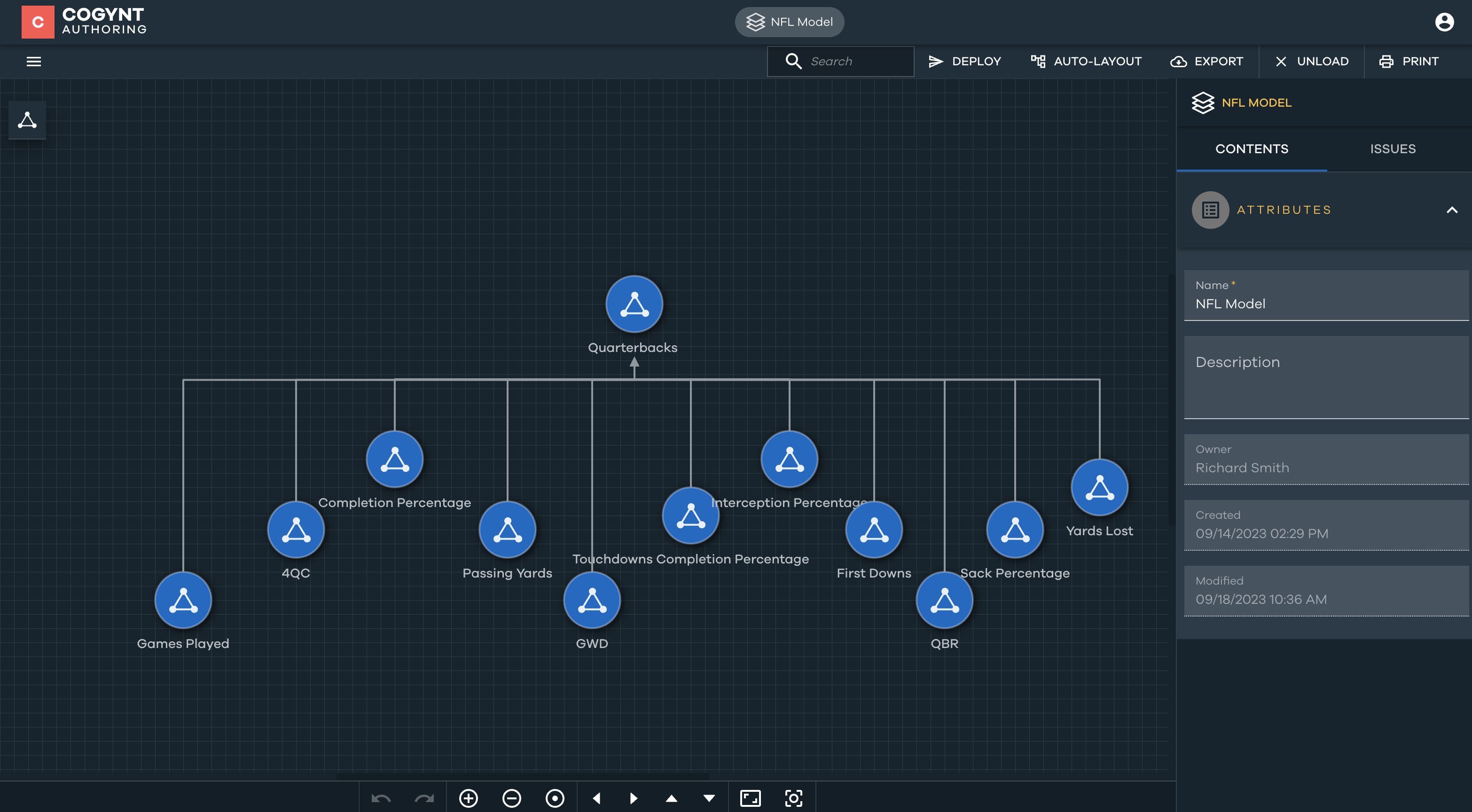
To start incorporating these into the model, do the following:
- Create an event pattern node for each of these statistics.
- Create one more event pattern node, called
Quarterbacks, to store their eventual outputs.
Configuring Event Pattern Logic
Now we need to set up the logic for each of the pattern nodes we've made.
In essence, we want each statistic to tell us a story: Based on that single stat, how risky is the QB? For each stat, we're going to show Cogynt what risky and less-risky QBs look like.
We will then have Cogynt gather each node's individual findings, and send them to the Quarterbacks node, where we'll calculate an overall risk score for the QB.
For step-by-step instructions about setting up event pattern logic, refer to Event Pattern Authoring and Outcome Computations Authoring in the Cogynt Authoring User Guide.
Games Played
They say that availability is the best ability. After all, the best QB in the league won't do your team much good if he isn't playing.
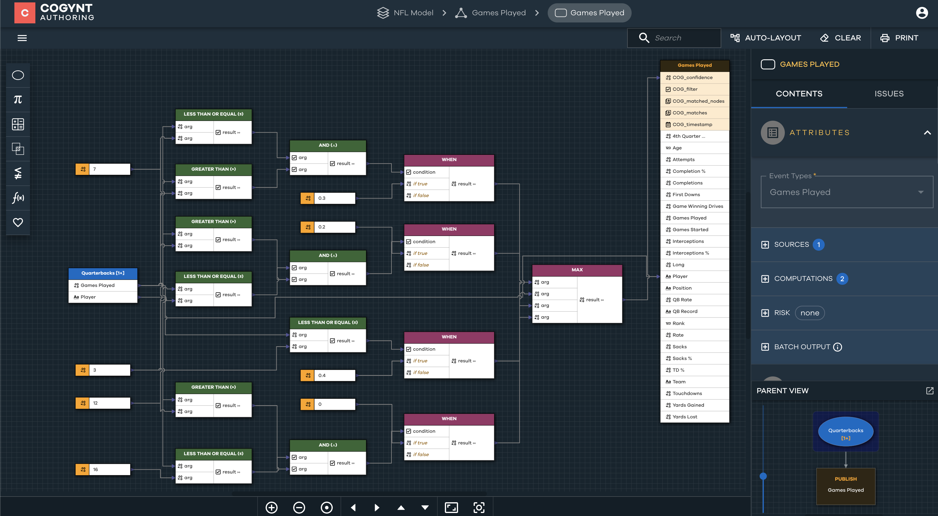
Accordingly, in the Games Played event pattern node, we should set up the node to show that the more games a QB plays in a season, the less risky he is. Conversely, the more games he misses, the riskier a proposition it is to sign him.
The node should contain the following logic:
- If the QB has played all 16 games of the season, their risk is 0.
- If the QB has played more than 12 games, their risk is 0. (This accounts for QBs who are given rest in meaningless games.)
- If the QB has played between 12 and 7 games, their risk is 0.2.
- If the QB has played between 7 and 3 games, their risk is 0.3.
- If the QB has played 3 or fewer games, their risk is 0.4.
4QC
Winning a football game is hard, but winning late in the game when you're trailing the other team is even harder. A good QB is able to fight back when trailing, especially when time is not on his side.
However, it's arguable that a great QB would play well enough not to find himself in such a situation too often. Our model should therefore avoiding grading a QB too harshly if he has no fourth-quarter comebacks to his name.
Our 4QC node should contain the following logic:
- If the QB has one or more fourth-quarter comebacks, their risk is 0.
- If the QB has less than one fourth-quarter comebacks, their risk is 0.1.
Completion Percentage
Passes help only if they find their intended receivers. We therefore want our model to reward QBs who complete a greater percentage of their passes.
Have the Completion Percentage node calculate the following:
- If the QB completed 100% of their passes, their risk is 0.
- If the QB completed between 100% and 61% of their passes, their risk is 0.
- If the QB completed between 60% and 31% of their passes, their risk is 0.2.
- If the QB completed 30% of their passes or fewer, their risk is 0.4.
Tip
For greater precision, try assigning a separate risk score for each 10% increase in completion percentage.
You can also try incorporating the number of pass attempts in your calculations.
Passing Yards
Not all passes are created equal. If a QB consistently hits receivers behind the line of scrimmage, only for the defense to tackle them before they can move downfield, then those passes aren't productive (even though they may elevate the QBs completion percentage).
To help account for this, we'll also track each QB's overall passing yards. The greater the number, the more effective the QB is at moving the ball down the field toward the endzone. Lower numbers correlate more strongly with weaker offensive performances.
Configure the Passing Yards node as follows:
- If the QB gained 6000 or more passing yards on the season, their risk is 0.
- If the QB gained between 6000 and 4001 passing yards on the season, their risk is 0.
- If the QB gained between 4000 and 2501 passing yards on the season, their risk is 0.2.
- If the QB gained less than 2500 yards on the season, their risk is 0.4.
GWD
The game-winning drive represents the highest-pressure situation possible: A must-score scenario where failure spells loss.
We want to give QBs credit for successfully completing a game-winning drive. However, we should avoid harshly penalizing QBs who do not have any. Like with the fourth-quarter comeback, strong QBs theoretically should not find themselves in a position where they must attempt a game-winning drive. (In practice, though, a lack of game-winning drives more likely means a QB fell short in his attempts.)
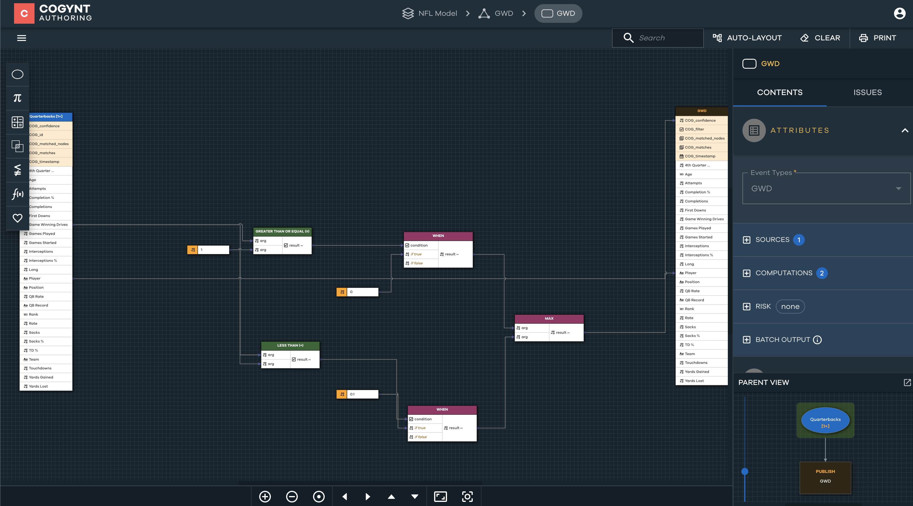
Build the GWD node with the following logic:
- If the QB has one or more game-winning drive, their risk is 0.
- If the QB has less than one game-winning drive, their risk is 0.1.
Tip
For additional modeling practice, try configuring the node to differentiate between QBs who didn't need game-winning drives, and QBs who did not succeed at attempted game-winning drives.
Touchdowns Completion Percentage
Ideally, a certain percentage of a QB's completed passes should end in a touchdown and generate points for the team. Games aren't scored based on yardage, after all.
With this in mind, let's tune our model so that QBs who achieve touchdowns with a certain regularity are considered safer bets, whereas QBs who generate fewer touchdowns as a result of their passes are noted as riskier propositions.
The Touchdowns Completion Percentage node should work as follows:
- If the QB's touchdowns completion percentage is greater than 10%, their risk is 0.
- If the QB's touchdowns completion percentage is less than 10% but greater than 4%, their risk is 0.
- If the QB's touchdowns completion percentage is less than or equal to 4%, but greater than 2%, then their risk is 0.1.
- If the QB's touchdowns completion percentage is 2% or less, their risk is 0.2.
Interception Percentage
Sometimes a pass ends up in the hands of the other team. This is a disastrous occurrence for the offense, as it grinds any drive to a halt, and often gives the opponent an easy opportunity to score. A QB's interception percentage gauges the frequency of such harmful passes, calculating interceptions as a percentage of their total number of pass attempts.
Given the high impact interceptions have on the game, our model needs to issue favorable marks to QBs who rarely throw interceptions, while also noting that QBs who frequently throw interceptions are risky to have under center.
Set up the Interception Percentage node so that:
- If the QB's interception percentage is 3% or less, their risk is 0.
- If the QB's interception percentage is between 3% and 5%, their risk is 0.1.
- If the QB's interception percentage is between 5% and 10%, their risk is 0.3.
- If the QB's interception percentage is greater than 10%, their risk is 0.4.
First Downs
First downs provide another way to assess whether a QB moves the ball effectively. A higher number of first downs indicates a greater ability to advance against opposing defenses. In the opposite direction, a lower number of first downs tends to correlate with defenses getting the better of the QB.
Configure the First Downs node as follows:
- If the QB has over 250 first downs, their risk is 0.
- If the QB has between 250 and 101 first downs, their risk is 0.
- If the QB has between 100 and 50 first downs, their risk is 0.1.
- If the QB has fewer than 50 first downs, their risk is 0.2.
QBR
The quarterback rating (QBR) evaluates all of a quarterback's contributions to the game. For more information about how QBR is calculated, refer to ESPN's explainer article.
For now, it's enough to say that a higher QBR indicates better QB play, whereas a lower number indicates poorer play.
Give the QBR node the following logic:
- If the QB has a QBR over 100, their risk is 0.
- If the QB has a QBR of less than or equal to 100, but greater than 80, their risk is 0.
- If the QB has a QBR of less than or equal to 80, but greater than 50, their risk is 0.2.
- If the QB has a QBR of less than or equal to 50, but greater than 30, their risk is 0.3.
- If the QB has a QBR of 30 or less, their risk is 0.4.
Sack Percentage
A QB is sacked when a player on defense manages to tackle them before they can generate a positive play. Although they're not usually as damaging as interceptions, a sack nonetheless represents an especially poor outcome for a QB.
Our model reviews the number of sacks a QB sustains as a percentage of the number of snaps they play. A higher sack rate means more of the QB's plays end in sacks, indicating a riskier QB prospect (both from a performance and injury perspective).
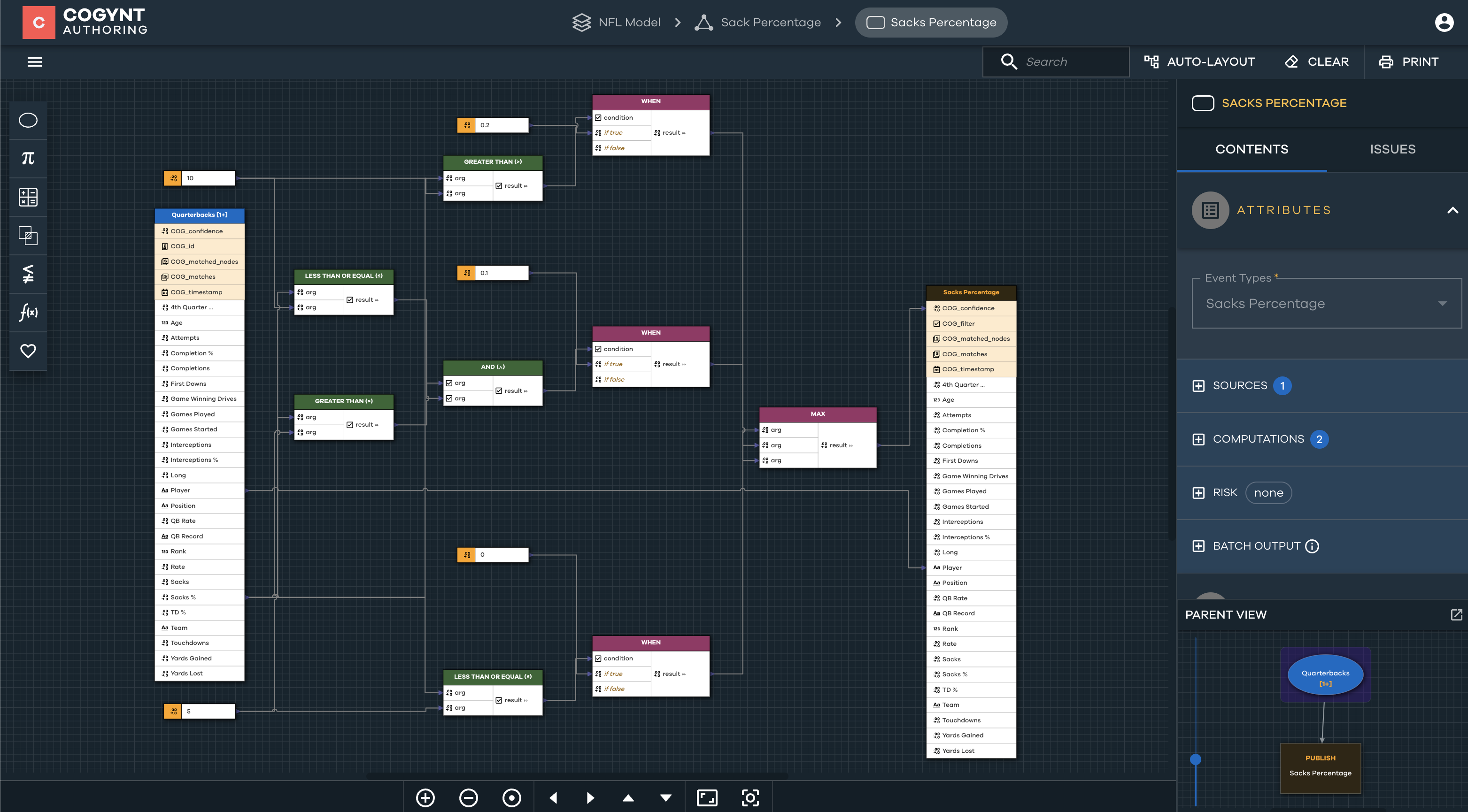
The Sack Percentage node should have the following logic:
- If the QB's sack percentage is less than or equal to 5%, their risk is 0.
- If the QB's sack percentage is greater than 5%, but less than or equal to 10%, their risk is 0.1.
- If the QB's sack percentage is greater than 10%, their risk is 0.2.
Yards Lost
Some sacks are worse than others. Being downed a yard behind the line of scrimmage is nowhere near as damaging to an offense as being downed ten or more yards behind it. The ability to minimize lost yardage due to such plays is a key skill for QBs.
Our model looks at how many yards a QB has lost over the course of a season, noting that QBs who lose more yards tend to be riskier roster choices.
Configure the Yards Lost node as follows:
- If the QB has lost 100 yards or fewer, their risk is 0.
- If the QB has lost between 100 and 150 yards, their risk is 0.1.
- If the QB has lost 150 yards or more, their risk is 0.2.
Reviewing Model Findings
Once your model is finished, you can ingest your data into Cogynt Workstation and build a view to examine your model's findings.
The following image shows our model's determinations for 2020 QB risk based on their 2019 performance.
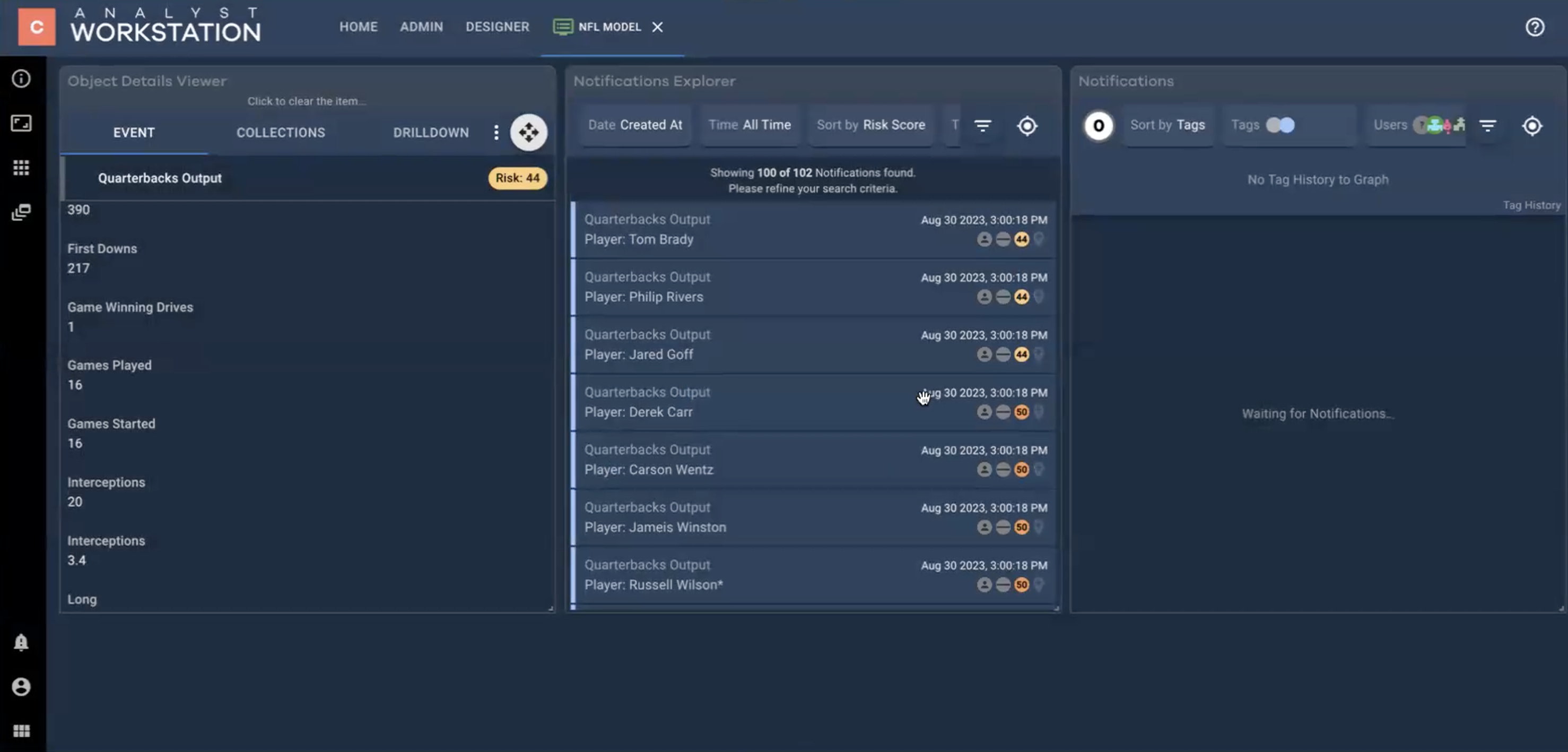
How did our model's top three QBs actually fare in 2020?
- Tom Brady, whom our model rated as the least risky QB, ended up winning the Super Bowl at the end of the 2020 season, piloting the Tampa Bay Buccaneers to a 31-9 victory over the defending champion Kansas City Chiefs.
- Jared Goff threw 22 TDs and 13 INTs en route to a 10-6 record for the LA Rams. He earned a playoff victory in the Wild Card round over the Seattle Seahawks (winning 30-20), but lost in the Divisional round to the Green Bay Packers (18-32).
- Philip Rivers led the Indianapolis Colts to a respectable 11-5 record, posting 24 TDs and 11 INTs.
Further Improvements
To develop this model further, try adding the following functionality:
- Aim for greater precision: To keep this model small and make it quicker for you to build, we've used broad strokes when accounting for QB performance. (For example, a 2501-yard passer is graded the same as a 4000-yard passer.) Try adding more intervals to the ranges for the various QB performance metrics, each with their own specific risk calculations, and see how it sharpens the picture of QB risk.
- Incorporate additional statistics: Are there any other data points that you think could offer a clearer picture of QB risk? Try incorporating them into the model.
- Analyze running back (RB) performance: Configure the model to account for an RB's touches, yards per carry, fumbles lost, and other relevant stats. Can your model identify the best RB of the bunch?
- Analyze wide receiver (WR) performance: Consider the kinds of statistics and variables that go into gauging a good WR. (For example, touchdowns, receptions, and yards after catch.) Track these values for the league's WRs, and see who's performing the best.
- Factor teammate performance into player analysis: Is a player being carried by his team? Or are his teammates holding him back? See if you can make the model determine how (or whether) one player's performance impacts another.
- Automatically update player analysis as season progresses: Take advantage of Cogynt's abilities to process continuous data streams so that the model automatically recalculates everything as the season goes on, or as multiple seasons pile up.